How Many Boxes are on the Trailer?
I recently came across an interesting puzzle:
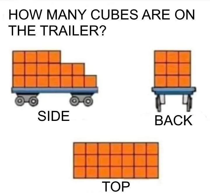
Without shading or a 3D-view, we can not give a definitive answer. Taking a look at the side view, we can give an upper bound. If we expect, from the side view, every visible cube to have two invisible boxes behind it, we get to 51 cubes. But what is the lower bound?
I thought, it would be a good idea and exercise, to solve this problem using a constraint solver. First I needed to decide on a model. As there exists a grid of \(7*3*3\) fields where each contains either a box or it does not. That sounds suspiciously like something Boolean. So let's model it as a Boolean satisfiability problem (SAT).
Since I haven't before, I wanted to try out PySAT and take it for a spin: The SAT solvers work with Boolean variables without names, just numbers. Additionally, our interface will create additional variables when we create more complex formulas due to Tseytin transformation. Tseytin transformation essentially creates a variable representing a subformula and the constraints for equivalence between the valuation of the newly created variable and the subformula. If you now want to create a new formula that contains the original formula as a subformula, you can refer to the single newly created variable, representing the whole subformula.
Because, as I said, the interface with the solver will be numbers-based, we need to decide on some representation or indexing between the solver's variables and our domain. We'll use a namedtuple for a Position P on the trailer, where x is along the depth of the trailer when viewed from the back, y is along the width of the trailer when viewed from the back, and z is along the height of the trailer, with the origin being at the bottom front left. We also need an empty list of constraints that we add to along the way:
from pysat.formula import *
from collections import namedtuple

P = namedtuple('P', ['x', 'y', 'z'])

boxes = {}

depth = 7
width = 3
height = 3

for x in range(depth):
  for y in range(width):
    for z in range(height):
      boxes[(x,y,z)] = Atom(P(x,y,z))

constraints = []
Instead of a namedtuple i initially wanted to use anonymous 3-tuples, but a bug in the library prevented me from doing that.
First we want to create the constraints for the side view. If we can see a box from that side, we know that at least one space in that group of 3 is filled by a box. We can simply use a disjunction over those three variables. If the space is empty, we know that there are no boxes. We can negate the disjunction. We "draw" the shape to make sure we got it right:
# side view
X = True
O = False
side_view = [
  [X,X,X,X,O,O,O],
  [X,X,X,X,X,X,O],
  [X,X,X,X,X,X,X],
]
for x in range(depth):
  for z in range(height):
    if side_view[-z-1][x]:
      constraints.append(Or(*[boxes[(x,y,z)] for y in range(width)]))
    else:
      constraints.append(Neg(Or(*[boxes[(x,y,z)] for y in range(width)])))
For the top view and back view we do not need to draw the shape that we are seeing, because every row/column/stack has a box in it and we do not need to consider the other case.
# back view
for y in range(width):
  for z in range(height):
    constraints.append(Or(*[boxes[(x,y,z)] for x in range(depth)]))

# top view
for y in range(width):
  for x in range(depth):
    constraints.append(Or(*[boxes[(x,y,z)] for z in range(height)]))
This looks like we are finished, but we have not yet considered gravity. If a box is anywhere not on the bottom level, it has to have another box under it. That is an implication:
# gravity
for x in range(depth):
  for y in range(width):
    for z in range(height-1):
      constraints.append(Implies(boxes[(x,y,z+1)], boxes[(x,y,z)]))
When I tried this out initially, there was a bug in the pySAT library where you could not use implications that are not on the top-level. This has been fixed quite fast.
Now we want to know the minimum number of needed boxes. We will get one solution, check how many boxes we needed, and add a constraint that we want one box less. We will do this until our formula is no longer satisfiable.
f = And(*constraints)

from pysat.solvers import Solver
with Solver(bootstrap_with=f) as solver:
  while solver.solve():
    model = solver.get_model()
    atoms = Formula.formulas((b for b in model if b > 0), atoms_only=True)
    boxes_needed = len(atoms)
    print("Solution with", boxes_needed, "boxes found")
    print(atoms)
    print("="*80)

    from pysat.card import CardEnc
    solver.append_formula(CardEnc.atmost(f.literals(boxes.values()), boxes_needed-1, vpool=Formula.export_vpool()))
It is important, when counting boxes, that we only extract the formulas/atoms that we created and not the ones created internally due to Tseyitin transformation. We count them and add a cardinality constraint, where we say, that we want at most one box less than we currently have used. An after only three iterations we get the following result:
Solution with 33 boxes found
[Atom(P(x=0, y=0, z=0)), Atom(P(x=0, y=1, z=0)), Atom(P(x=0, y=2, z=0)), Atom(P(x=0, y=1, z=1)), Atom(P(x=0, y=2, z=1)), Atom(P(x=0, y=1, z=2)), Atom(P(x=0, y=2, z=2)), Atom(P(x=1, y=0, z=0)), Atom(P(x=1, y=1, z=0)), Atom(P(x=1, y=2, z=0)), Atom(P(x=1, y=0, z=1)), Atom(P(x=1, y=0, z=2)), Atom(P(x=2, y=0, z=0)), Atom(P(x=2, y=1, z=0)), Atom(P(x=2, y=2, z=0)), Atom(P(x=2, y=0, z=1)), Atom(P(x=2, y=0, z=2)), Atom(P(x=3, y=0, z=0)), Atom(P(x=3, y=1, z=0)), Atom(P(x=3, y=2, z=0)), Atom(P(x=3, y=0, z=1)), Atom(P(x=3, y=0, z=2)), Atom(P(x=4, y=0, z=0)), Atom(P(x=4, y=1, z=0)), Atom(P(x=4, y=2, z=0)), Atom(P(x=4, y=0, z=1)), Atom(P(x=5, y=0, z=0)), Atom(P(x=5, y=1, z=0)), Atom(P(x=5, y=2, z=0)), Atom(P(x=5, y=0, z=1)), Atom(P(x=6, y=0, z=0)), Atom(P(x=6, y=1, z=0)), Atom(P(x=6, y=2, z=0))]
================================================================================
Solution with 32 boxes found
[Atom(P(x=0, y=0, z=0)), Atom(P(x=0, y=1, z=0)), Atom(P(x=0, y=2, z=0)), Atom(P(x=0, y=0, z=1)), Atom(P(x=0, y=0, z=2)), Atom(P(x=1, y=0, z=0)), Atom(P(x=1, y=1, z=0)), Atom(P(x=1, y=2, z=0)), Atom(P(x=1, y=1, z=1)), Atom(P(x=1, y=1, z=2)), Atom(P(x=2, y=0, z=0)), Atom(P(x=2, y=1, z=0)), Atom(P(x=2, y=2, z=0)), Atom(P(x=2, y=0, z=1)), Atom(P(x=2, y=2, z=1)), Atom(P(x=2, y=2, z=2)), Atom(P(x=3, y=0, z=0)), Atom(P(x=3, y=1, z=0)), Atom(P(x=3, y=2, z=0)), Atom(P(x=3, y=0, z=1)), Atom(P(x=3, y=0, z=2)), Atom(P(x=4, y=0, z=0)), Atom(P(x=4, y=1, z=0)), Atom(P(x=4, y=2, z=0)), Atom(P(x=4, y=2, z=1)), Atom(P(x=5, y=0, z=0)), Atom(P(x=5, y=1, z=0)), Atom(P(x=5, y=2, z=0)), Atom(P(x=5, y=2, z=1)), Atom(P(x=6, y=0, z=0)), Atom(P(x=6, y=1, z=0)), Atom(P(x=6, y=2, z=0))]
================================================================================
Solution with 31 boxes found
[Atom(P(x=0, y=0, z=0)), Atom(P(x=0, y=1, z=0)), Atom(P(x=0, y=2, z=0)), Atom(P(x=0, y=0, z=1)), Atom(P(x=0, y=0, z=2)), Atom(P(x=1, y=0, z=0)), Atom(P(x=1, y=1, z=0)), Atom(P(x=1, y=2, z=0)), Atom(P(x=1, y=2, z=1)), Atom(P(x=1, y=2, z=2)), Atom(P(x=2, y=0, z=0)), Atom(P(x=2, y=1, z=0)), Atom(P(x=2, y=2, z=0)), Atom(P(x=2, y=0, z=1)), Atom(P(x=2, y=0, z=2)), Atom(P(x=3, y=0, z=0)), Atom(P(x=3, y=1, z=0)), Atom(P(x=3, y=2, z=0)), Atom(P(x=3, y=1, z=1)), Atom(P(x=3, y=1, z=2)), Atom(P(x=4, y=0, z=0)), Atom(P(x=4, y=1, z=0)), Atom(P(x=4, y=2, z=0)), Atom(P(x=4, y=2, z=1)), Atom(P(x=5, y=0, z=0)), Atom(P(x=5, y=1, z=0)), Atom(P(x=5, y=2, z=0)), Atom(P(x=5, y=2, z=1)), Atom(P(x=6, y=0, z=0)), Atom(P(x=6, y=1, z=0)), Atom(P(x=6, y=2, z=0))]
================================================================================
Now we know that the lower bound on boxes is 31. But what does such a solution look like? Let us plot them using matplotlib, putting them all in a three-dimensional array
import matplotlib.pyplot as plt
import numpy as np

# Prepare some coordinates
x, y, z = np.indices((depth, depth, depth))

cubes = [((atom.object.x == x) & (atom.object.y == y) & (atom.object.z == z) )  for atom in atoms]

# Combine the objects into a single boolean array
voxelarray = cubes[0]
for cube in cubes[1:]:
  voxelarray |= cube

# Plot
fig, ax = plt.subplots(subplot_kw={"projection": "3d"})
ax.voxels(voxelarray, edgecolor='k')

ax.set(xticklabels=[], yticklabels=[], zticklabels=[])

plt.show()
And here is our trailer in glorius 3D:
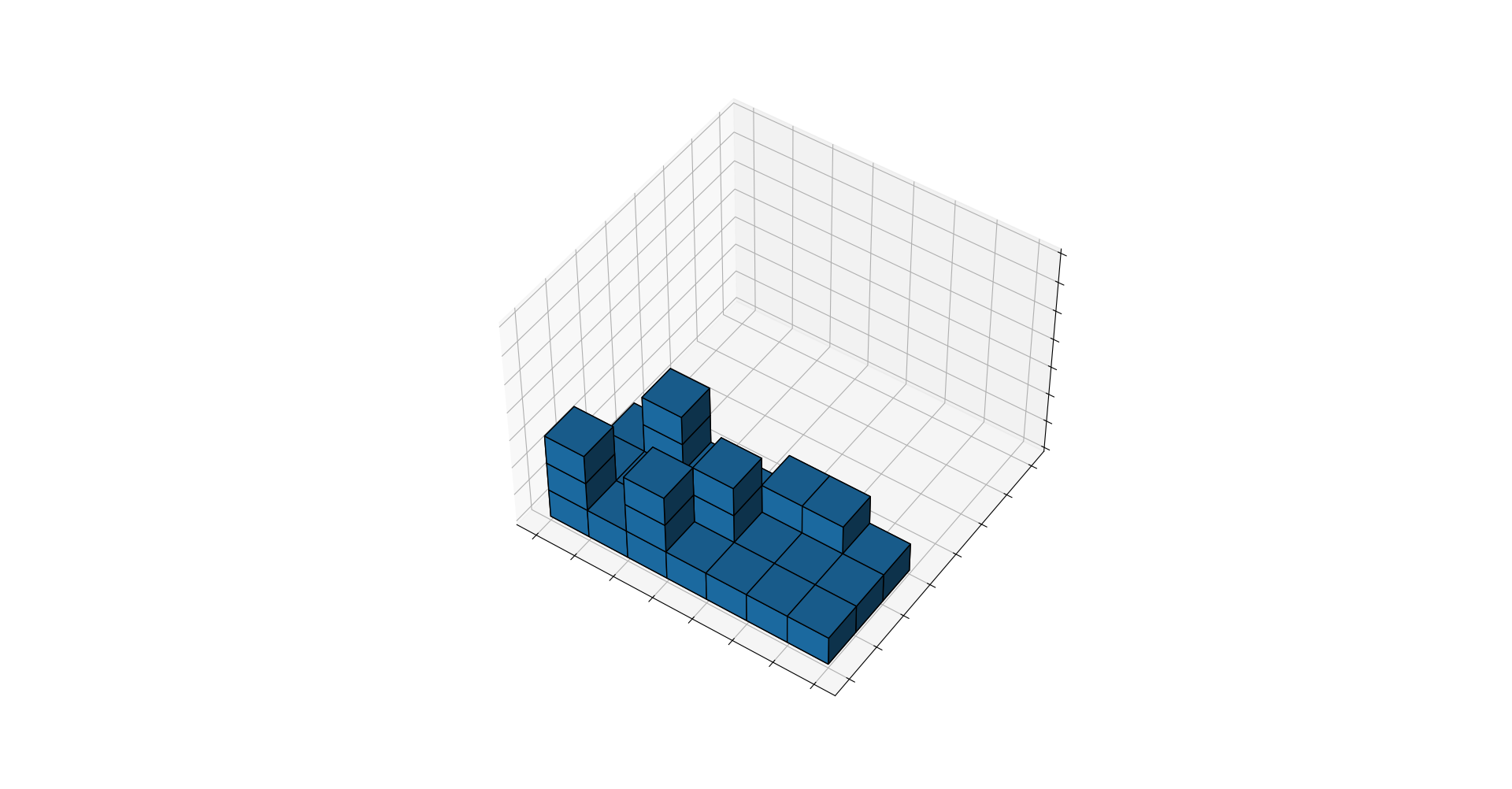
Obviously the solution is not unique, as some stacks can be swapped and the whole configuration can be mirrored.
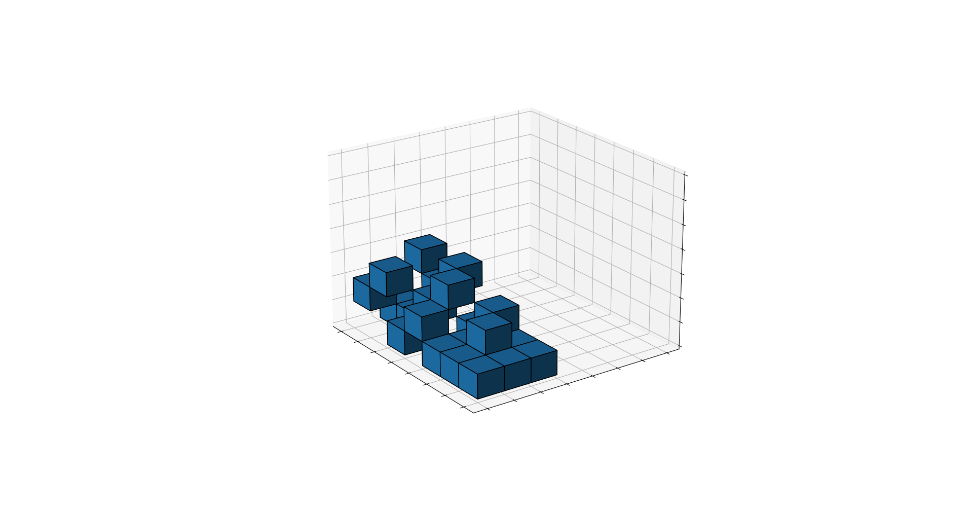
And just out of curiosity, if there were no gravity...
Solution with 26 boxes found
[Atom(P(x=0, y=0, z=0)), Atom(P(x=0, y=1, z=1)), Atom(P(x=0, y=2, z=1)), Atom(P(x=0, y=1, z=2)), Atom(P(x=0, y=2, z=2)), Atom(P(x=1, y=1, z=0)), Atom(P(x=1, y=2, z=0)), Atom(P(x=1, y=0, z=1)), Atom(P(x=1, y=0, z=2)), Atom(P(x=2, y=1, z=0)), Atom(P(x=2, y=2, z=0)), Atom(P(x=2, y=0, z=1)), Atom(P(x=2, y=0, z=2)), Atom(P(x=3, y=1, z=0)), Atom(P(x=3, y=2, z=0)), Atom(P(x=3, y=0, z=1)), Atom(P(x=3, y=0, z=2)), Atom(P(x=4, y=1, z=0)), Atom(P(x=4, y=2, z=0)), Atom(P(x=4, y=0, z=1)), Atom(P(x=5, y=1, z=0)), Atom(P(x=5, y=2, z=0)), Atom(P(x=5, y=0, z=1)), Atom(P(x=6, y=0, z=0)), Atom(P(x=6, y=1, z=0)), Atom(P(x=6, y=2, z=0))]
================================================================================
Solution with 25 boxes found
[Atom(P(x=0, y=2, z=0)), Atom(P(x=0, y=2, z=1)), Atom(P(x=0, y=0, z=2)), Atom(P(x=0, y=1, z=2)), Atom(P(x=1, y=2, z=0)), Atom(P(x=1, y=1, z=1)), Atom(P(x=1, y=0, z=2)), Atom(P(x=1, y=2, z=2)), Atom(P(x=2, y=2, z=0)), Atom(P(x=2, y=1, z=1)), Atom(P(x=2, y=0, z=2)), Atom(P(x=2, y=2, z=2)), Atom(P(x=3, y=2, z=0)), Atom(P(x=3, y=2, z=1)), Atom(P(x=3, y=0, z=2)), Atom(P(x=3, y=1, z=2)), Atom(P(x=4, y=1, z=0)), Atom(P(x=4, y=2, z=0)), Atom(P(x=4, y=0, z=1)), Atom(P(x=5, y=1, z=0)), Atom(P(x=5, y=2, z=0)), Atom(P(x=5, y=0, z=1)), Atom(P(x=6, y=0, z=0)), Atom(P(x=6, y=1, z=0)), Atom(P(x=6, y=2, z=0))]
================================================================================
Solution with 24 boxes found
[Atom(P(x=0, y=2, z=0)), Atom(P(x=0, y=2, z=1)), Atom(P(x=0, y=0, z=2)), Atom(P(x=0, y=1, z=2)), Atom(P(x=1, y=2, z=0)), Atom(P(x=1, y=1, z=1)), Atom(P(x=1, y=0, z=2)), Atom(P(x=1, y=2, z=2)), Atom(P(x=2, y=2, z=0)), Atom(P(x=2, y=1, z=1)), Atom(P(x=2, y=0, z=2)), Atom(P(x=2, y=2, z=2)), Atom(P(x=3, y=2, z=0)), Atom(P(x=3, y=1, z=1)), Atom(P(x=3, y=0, z=2)), Atom(P(x=4, y=1, z=0)), Atom(P(x=4, y=2, z=0)), Atom(P(x=4, y=0, z=1)), Atom(P(x=5, y=1, z=0)), Atom(P(x=5, y=2, z=0)), Atom(P(x=5, y=0, z=1)), Atom(P(x=6, y=0, z=0)), Atom(P(x=6, y=1, z=0)), Atom(P(x=6, y=2, z=0))]
================================================================================
Solution with 23 boxes found
[Atom(P(x=0, y=2, z=0)), Atom(P(x=0, y=2, z=1)), Atom(P(x=0, y=0, z=2)), Atom(P(x=0, y=1, z=2)), Atom(P(x=1, y=2, z=0)), Atom(P(x=1, y=1, z=1)), Atom(P(x=1, y=0, z=2)), Atom(P(x=1, y=2, z=2)), Atom(P(x=2, y=2, z=0)), Atom(P(x=2, y=1, z=1)), Atom(P(x=2, y=0, z=2)), Atom(P(x=3, y=2, z=0)), Atom(P(x=3, y=1, z=1)), Atom(P(x=3, y=0, z=2)), Atom(P(x=4, y=1, z=0)), Atom(P(x=4, y=2, z=0)), Atom(P(x=4, y=0, z=1)), Atom(P(x=5, y=1, z=0)), Atom(P(x=5, y=2, z=0)), Atom(P(x=5, y=0, z=1)), Atom(P(x=6, y=0, z=0)), Atom(P(x=6, y=1, z=0)), Atom(P(x=6, y=2, z=0))]
================================================================================
Solution with 22 boxes found
[Atom(P(x=0, y=2, z=0)), Atom(P(x=0, y=1, z=1)), Atom(P(x=0, y=0, z=2)), Atom(P(x=1, y=1, z=0)), Atom(P(x=1, y=0, z=1)), Atom(P(x=1, y=2, z=2)), Atom(P(x=2, y=0, z=0)), Atom(P(x=2, y=2, z=0)), Atom(P(x=2, y=0, z=1)), Atom(P(x=2, y=1, z=2)), Atom(P(x=3, y=0, z=0)), Atom(P(x=3, y=2, z=1)), Atom(P(x=3, y=1, z=2)), Atom(P(x=4, y=0, z=0)), Atom(P(x=4, y=2, z=0)), Atom(P(x=4, y=1, z=1)), Atom(P(x=5, y=1, z=0)), Atom(P(x=5, y=2, z=0)), Atom(P(x=5, y=0, z=1)), Atom(P(x=6, y=0, z=0)), Atom(P(x=6, y=1, z=0)), Atom(P(x=6, y=2, z=0))]
================================================================================
Solution with 21 boxes found
[Atom(P(x=0, y=1, z=0)), Atom(P(x=0, y=0, z=1)), Atom(P(x=0, y=2, z=2)), Atom(P(x=1, y=1, z=0)), Atom(P(x=1, y=2, z=1)), Atom(P(x=1, y=0, z=2)), Atom(P(x=2, y=0, z=0)), Atom(P(x=2, y=1, z=1)), Atom(P(x=2, y=2, z=2)), Atom(P(x=3, y=2, z=0)), Atom(P(x=3, y=0, z=1)), Atom(P(x=3, y=1, z=2)), Atom(P(x=4, y=0, z=0)), Atom(P(x=4, y=1, z=0)), Atom(P(x=4, y=2, z=1)), Atom(P(x=5, y=0, z=0)), Atom(P(x=5, y=2, z=0)), Atom(P(x=5, y=1, z=1)), Atom(P(x=6, y=0, z=0)), Atom(P(x=6, y=1, z=0)), Atom(P(x=6, y=2, z=0))]
================================================================================